The Comparison Of Distributions – Employing Affine Transformations To Assess Risk And Return
Friday, 26 February 2016By Con Keating
The companion blog to this article is an extensive description of a new method (affine transformation) of comparing distributions, which is the central analytic problem when evaluating fund manager performance.
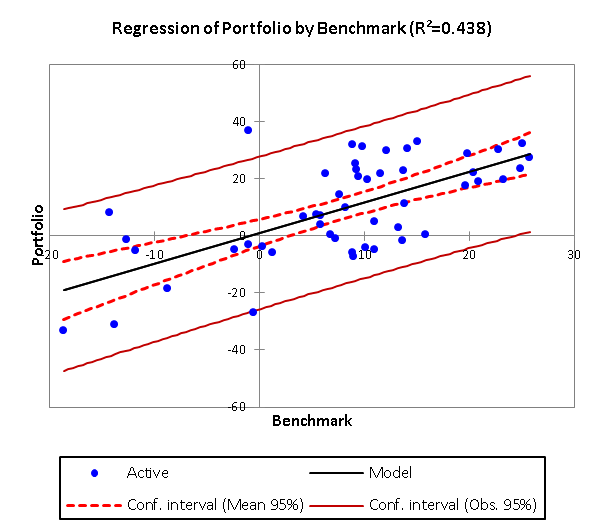
The usual and most widely used method, the alpha and beta of the capital asset pricing model (CAPM), is unsatisfactory in many regards, not least the low confidence that applies to estimates. We illustrate this issue in figure 1 for the returns of an arbitrary Portfolio and Benchmark using a standard ordinary least squares regression. The descriptive statistics for these two returns distributions are:
| Statistic | Benchmark | Portfolio |
|---|---|---|
| No. of Observations | 50.00 | 50.00 |
| Minimum | -18.65 | -33.29 |
| Maximum | 25.73 | 36.94 |
| 1st Quartile | 4.54 | -2.62 |
| Median | 9.22 | 8.97 |
| 3rd Quartile | 13.80 | 23.10 |
| Mean | 8.12 | 9.81 |
| Variance (n-1) | 113.09 | 299.18 |
| Standard deviation (n-1) | 10.63 | 17.30 |
| Skewness (Pearson) | -0.62 | -0.52 |
| Kurtosis (Pearson) | 0.11 | -0.28 |
Table 1: Descriptive Statistics for Returns Distributions
Two points stand out from these statistics: first, that the Portfolio is very significantly more volatile than the Benchmark, and second that the median lies above the mean for the Benchmark while lying below for the Portfolio.

The numerical values of the intercept and slope, and elementary diagnostic statistics, of this regression line are:
| Source | Value | Standard Error | t | Pr > |t| | Lower bound (95%) | Upper bound (95%) |
|---|---|---|---|---|---|---|
| Intercept (Alpha) | 1.066 | 2.340 | 0.456 | 0.651 | -3.639 | 5.771 |
| Benchmark (Beta) | 1.076 | 0.176 | 6.117 | < 0.0001 | 0.723 | 1.430 |
Table 2: OLS Regression estimates for Portfolio on Benchmark.
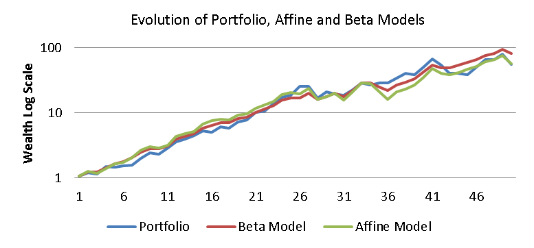
The estimate of Alpha, at 1.066%, for the Portfolio is highly uncertain, bounded at the 95% level in the range -3.639% to 5.771%. This implies that we can really say very little about the fund manager’s production of risk-free returns. Perhaps more surprising, given the differences observed in the earlier ranges of returns and standard deviations, is that the portfolio does not appear to be highly leveraged (Beta) at 1.076 times the Benchmark. This is not a case of misestimating the value of the series Beta; using the standard analytic series estimator, β = ρPB (σρ ÷ σB), returns the same 1.07 value. The issue here is that a series having these estimated parameters does not represent the Portfolio meaningfully or faithfully. By way of indication of this discrepancy, the geometric return of the (Beta) modelled portfolio over the 50-year period is 9.19%, which far exceeds the compound 8.36% of the original portfolio. The evolution of the wealth process for the Portfolio and for the Beta and (proposed) Affine models is shown as figure 2.

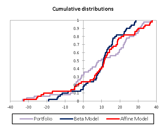
The differences in the distributions of returns for the Portfolio and both models are perhaps easier to observe directly, as figure 3 shows. The markedly lower variability of the Beta model is immediately obvious – a standard deviation of 11.45% versus 17.30% for the Portfolio. Similarity of the variance of the Portfolio and Beta Model is formally rejected by all commonly used tests (Fisher, Levene and Bartlett).
Formal testing, using the Kolmogorov-Smirnov statistic, of the hypothesis that the Beta model and the Affine model outcomes share a common distribution with the Portfolio result in acceptance of this hypothesis for the Affine model, but rejection of it for the Beta. The clearest implication of this analysis is that the standard Beta model may be a very poor representation of a Portfolio.

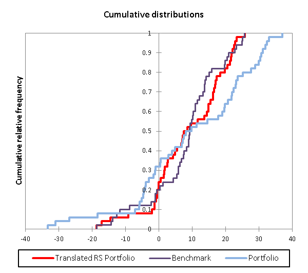
The approach advocated for distribution comparison is affine transformation, which despite the obscurity of that expression, is a simple mathematical operation. It consists of rescaling and translating the Portfolio returns distribution such that it shares a common range of support with the Benchmark. This process is explained in greater detail in the accompanying blog, but is illustrated here as figure 4. The original Portfolio returns (light blue) become the rescaled and translated returns (red).

The interpretation of the affine transformation is direct: the translation of the distribution is a measure of risk-free value added, and the rescaling factor a measure of leverage, and finally, once sharing a common support, differences between the means of the two distributions are sufficient for value added performance assessment, including skill.
In essence, translation separates the investment process into risk-free and risky elements, separating the questions of location and risk or return distribution management. For these datasets, under this approach, for the Portfolio the alpha (translation) is negative (-2.39%), the beta, leverage or rescaling factor is large (1.58 times) and the skill positive at 46 basis points. These values are markedly different from the earlier CAPM estimation, but are intuitively more appealing and statistically more significant.
This approach to distribution comparison or performance evaluation also offers several new insights into methods of risk and return management, in the simplest and most intuitive of worlds, where risk and return are merely loss and gain.