The Comparison Of Distributions
Thursday, 25 February 2016By Con Keating
In mathematics, there is no general method for the comparison of functions, in large part because of the richness and complexity of their forms. However, simple functions, such as probability density functions, may be compared by a technique known as affine transformation - that is by translation and rescaling, or vice versa. The comparison of distribution functions is a recurrent problem in financial analysis – for example, in the evaluation of performance in portfolio management.
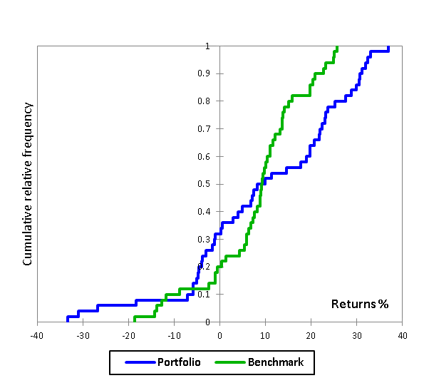
As these terms hold little intuitive meaning for the non-mathematician, we illustrate first the problem, and then, by stages, exactly what is taking place in an affine transformation. The two distributions we wish to compare are shown in figure 1.

While we have labelled these two returns distributions as portfolio and benchmark, they are simply two arbitrary distributions for comparison. It is not at all obvious which is preferable or superior; to illustrate this point, the geometric (compound) return of the portfolio is significantly better that the benchmark, but the information ratio (mean return divided by volatility, which is taken to be the standard deviation) shows the benchmark to be preferable ( 0.71 versus 0.48). The descriptive statistics for these distributions are:
| Portfolio | Benchmark | |
|---|---|---|
| Max | 36.94 | 25.73 |
| Min | -33.29 | -18.65 |
| Mean | 9.81 | 8.12 |
| Geo Mean | 8.36 | 7.58 |
| St Dev | 17.30 | 10.63 |
| Range | 70.24 | 44.38 |
Table 1: Descriptive statistics for Benchmark and Portfolio
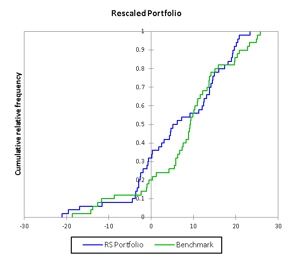
The first stage of the affine transformation is rescaling. This is modification of the portfolio returns distribution such that it has the same range of returns as the Benchmark. The rescaling factor is simply the ratio of the ranges of the two distributions. In this case therefore, the observed benchmark range is 25.73- (-18.65) i.e. 44.38, and that of the portfolio is 36.94-(-33.29) i.e. 70.23; so that the scaling factor is 44.38/70.23, or .632. This transformation is closely equivalent to indexing two or more series to the same base, which allows for comparisons of the rate of change between the series. The difference here is that instead of having a single base, the series have two anchors in common, which allows for a comparison of how they behave as a whole, relative to each other, within that range.

Rescaling alters the descriptive statistics of the portfolio, as is shown in table 2.
| Portfolio | Benchmark | Rescaled Portfolio | |
|---|---|---|---|
| Max | 36.94 | 25.73 | 23.34 |
| Min | -33.29 | -18.65 | -21.04 |
| Mean | 9.81 | 8.12 | 6.20 |
| Geo Mean | 8.36 | 7.58 | 5.62 |
| St Dev | 17.30 | 10.63 | 10.93 |
| Range | 70.24 | 44.38 | 44.38 |
Table 2: Descriptive Statistics after Portfolio Rescaling
Notice that the Geometric Mean of the rescaled portfolio is not the previous Geometric Mean scaled by 0.632.
There is a simple interpretation of rescaling as the leverage, gearing or “Beta” of the Portfolio relative to the Benchmark. In other words, the leverage of the Portfolio relative to the Benchmark is a measure of the relative range. In as much as the Portfolio range of returns is greater than that of the Benchmark, its leverage is the reciprocal of the scaling factor, i.e. 1/.6319, or 1.5826.
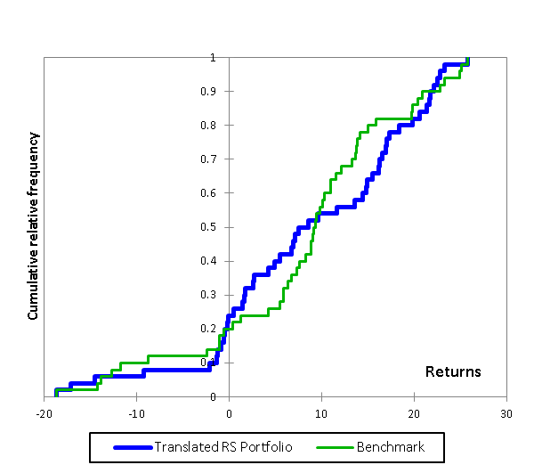
The final step in the affine transformation is translation of the rescaled portfolio distribution such that it shares a common range of support with the Benchmark. This involves adding, in this case, a fixed amount to each element of the rescaled portfolio returns distribution. In this instance we effectively are shifting the portfolio returns to the right, so that not only do these returns share the same range as that of the benchmark, but now also the same start and end values (i.e. minimum and maximum values).

It is important to note that translation preserves the shape of the portfolio distribution and is therefore a riskless operation. With shape preserved, it is riskless. With roots in the capital asset pricing model, risk-free terms are usually known as “Alpha” (α). In this affine set-up, it is simply a measure of the location of a distribution, but outside of the distribution and its risk characteristics. In this case, the value of translation term (or alpha) is positive (2.39%), but as the portfolio is located below the Benchmark, this represents negative value added for the Portfolio relative to the Benchmark.
With the (translated and rescaled) Portfolio and Benchmark sharing a common range of support, we may compare them directly by comparing their mean returns (B 8.12% versus TRS Portfolio 8.59%) which indicates that the translated and rescaled Portfolio returns 46 basis points more than the Benchmark. While this may be interpreted as manager skill, this would be subject to the criticism that the alpha or location of the portfolio was far more removed. It should be noted that everywhere here we are comparing returns, in a completely intuitive way. Portfolio value-added measurement is simple addition.
Some Important Insights
The first is that true alpha generation, uniformly increasing the amount of each return, would prove extremely difficult or impossible to achieve in practice. All other alterations to returns alter the shape of the distribution and with that, its risk profile.
We are also able to distinguish between returns occurring within a distribution range and those occurring outside of it. The latter affect the rescaling or leverage factor. This can provide significant further insights for risk management, but we leave those aspects for later papers. Immediately, we shall consider the relation between the compound or geometric return and the simple arithmetic mean.
The original portfolio had an arithmetic mean of 9.81% and a geometric mean of 8.36%. The majority of this difference (1.50%) is explained by the variance term of the expansion. This is the standard first order adjustment to arithmetic average returns when estimating the geometric mean return. In this case, higher order moments add 5 basis points to the geometric return. It is notable that though many analysts place much emphasis on higher moments, such as skewness and kurtosis, they are usually of low importance in the realised total returns of portfolios (or benchmarks). By contrast, the benchmark has all but 2 basis points of the difference (again positive) between its arithmetic and geometric mean accounted for by the higher moments of its distribution. After affine transformation, the Portfolio has just 2 basis points of the difference between its geometric and arithmetic returns unexplained. The adjustments due to variance are 56 basis points in the case of the benchmark and 59 basis points in the case of the affine transformed Portfolio.
Altering any of returns lying between the minimum and maximum, provided these alterations do not change the minimum or maximum, is uninteresting and very much the substance of standard risk and return analysis. This is inside risk management. In fact, because these inside alterations lie within the range of support, the variance and higher moments are bounded, but in the interest of brevity, further consideration of that will be omitted here.
However alteration to returns which affect the minimum or maximum result in complex trade-offs between the rescaling and translation terms, and with that the make-up of the portfolio value-added. We shall now examine, in turn, the effects of increasing the minimum return and the highest return.
Suppose we begin by increasing the lowest return such that it is equal to the second lowest. The addition of 2.38% to the minimum makes the new minimum -30.93. This increases the rescaling factor to 0.6359 ( or leverage of 1.5294) since it reduces the range of the portfolio. The descriptive statistics of the new rescaled Portfolio and the Benchmark are shown in table 3.
| Min Increased | Benchmark | Minimum Increased Rescaled | |
|---|---|---|---|
| Max | 36.94 | 25.73 | 24.15 |
| Min | -30.93 | -18.65 | -20.22 |
| Mean | 9.86 | 8.12 | 6.44 |
| St Dev | 17.18 | 10.63 | 11.23 |
| Range | 67.88 | 44.38 | 44.38 |
Table 3: Descriptive statistics minimum increased rescaled Portfolio
The alpha has been increased from the earlier -2.39% to -1.58%. Note that adding 2.38% to the minimum, as here, does not increase the alpha by this amount – that would require 2.38% to be added to all returns. The rescaled portfolio arithmetic return is now 6.44% versus the previous 6.20%. However, manager skill or luck relative to the benchmark mean return (8.12 -(6.44 + 1.58) = -.10) is now -10 basis points.
If we continue the process by adding to the two lowest returns (Portfolio 2), such that the portfolio minimum is now -26.81, then the rescaling factor further increases to 0.69616 (or a leverage of 1.4365), and we have added a total of 10.61% to these two lowest returns. The descriptive statistics for this portfolio and its rescaled version are shown as table 4. The alpha is now -1 basis point and the manager valued added or skill now becomes -1.13% - even after adding 10.61% to the total returns.
| Portfolio 2 | Benchmark | Rescaled Portfolio 2 | |
|---|---|---|---|
| Max | 36.94 | 25.73 | 25.72 |
| Min | -26.81 | -18.65 | -18.66 |
| Mean | 10.02 | 8.12 | 6.98 |
| St Dev | 16.79 | 10.63 | 11.69 |
| Range | 63.75 | 44.38 | 44.38 |
Table 4: Descriptive statistics Portfolio 2
It is difficult to describe these results as anything other than contra-intuitive and difficult, but progressively adding to the minimum returns has raised alpha but lowered the manager skill or luck attribute, in ways that are not at all obvious.
Adding to the maximum return also alters the range of the portfolio distribution and with that the rescaling factor and rescaled distribution. For this illustration, we add the same amount (2.38%) to the largest return as was used for the original minimum alteration. The rescaling factor becomes 0.61138 (or a leverage of 1.63590), and the descriptive statistics for the new portfolio and its rescaled version are shown as table 5.
| Portfolio 2 | Benchmark | Rescaled Portfolio 2 | |
|---|---|---|---|
| Max | 39.30 | 25.73 | |
| Min | -33.29 | -18.65 | |
| Mean | 9.86 | 8.12 | |
| St Dev | 17.38 | 10.63 | |
| Range | 72.60 | 44.38 |
Table 5: Portfolio 2 high return
The effect of adding a 2.38% return to the maximum shifts the alpha to -1.70 from the initial -2.39% and differs from the effect of adding this amount to the minimum return, which was to -1.58%. The manager skill or luck is now -39 basis points, (6.03 + 1.70 = 7.73 – 8.12 = -.39), which in the lower case was -10 basis points.
The central insight here is that not all returns are equal in effect. Total value added in the base case was -1.92% (-2.39+ 0.46),with leverage of 1.5826. The addition of 2.38% to the minimum return made this total -1.68%, (-1.58 – 0.10),with leverage of 1.5295, but adding the same amount to the highest return makes the total value added -2.09 (-1.70 – 0.39), with leverage of 1.6359, which is both higher than both the lower-altered, and the original portfolio. This latter result is deeply contra-intuitive, but adding extra return to the highest return can lower value-added by increasing gearing.
Conclusions
The method illustrated in this article is simple mathematics, but offers much by way of insight into portfolio risk and return management. The familiar capital asset pricing model with its alpha and beta is merely a variant to this affine transformation, although one that is replete with economic assumptions and models (see blog). It is evident that though the mathematical techniques are elementary, the question of investment performance evaluation is a complex and often contra-intuitive affair, and that the standard capital asset pricing model approach obscures rather more than it illuminates.
The method can also be used to unpack many currently popular fund management techniques, such as smart beta, as well as the effects of costs and charges in value for money analysis.